


On this article, you’ll discover ways to consider k-means clustering outcomes utilizing silhouette evaluation and interpret each common and per-cluster scores to information mannequin decisions.
Subjects we’ll cowl embrace:
What the silhouette rating measures and find out how to compute it
Tips on how to use silhouette evaluation to choose an inexpensive variety of clusters
Visualizing per-sample silhouettes to diagnose cluster high quality
Right here’s the way it works.

Okay-Means Cluster Analysis with Silhouette Evaluation
Picture by Editor
Introduction
Clustering fashions in machine studying should be assessed by how properly they separate knowledge into significant teams with distinctive traits. One of many key metrics for evaluating the interior cohesion and mutual separation of clusters produced by iterative algorithms like k-means is the silhouette rating, which quantifies how comparable an object — an information occasion i — is to its personal cluster in comparison with different clusters.
This text focuses on find out how to consider and interpret cluster high quality via silhouette evaluation, that’s, an evaluation of cluster construction and validity based mostly on disciplined use of the silhouette metric. Silhouette evaluation has sensible implications in real-world segmentation duties throughout advertising, prescribed drugs, chemical engineering, and extra.
Understanding the Silhouette Metric
Given an information level or occasion i in a dataset that has been partitioned into okay clusters, its silhouette rating is outlined as:
[ s(i) = frac{b(i) – a(i)}{max{a(i), b(i)}} ]
Within the components, a(i) is the intra-cluster cohesion, that’s, the typical distance between i and the remainder of the factors within the cluster it belongs to. In the meantime, b(i) is the inter-cluster separation, specifically, the typical distance between i and the factors within the closest neighboring cluster.
The silhouette rating ranges from −1 to 1. Decrease a(i) and better b(i) values contribute to a better silhouette rating, which is interpreted as higher-quality clustering, with factors strongly tied to their cluster and properly separated from different clusters. In sum, the upper the silhouette rating, the higher.
In observe, we sometimes compute the typical silhouette rating throughout all situations to summarize cluster high quality for a given answer.
The silhouette rating is extensively used to guage cluster high quality in various datasets and domains as a result of it captures each cohesion and separation. It is usually helpful, as a substitute or a complement to the Elbow Methodology, for choosing an applicable variety of clusters okay — a needed step when making use of iterative strategies like k-means and its variants.
Moreover, the silhouette rating doubles as an insightful visible assist whenever you plot particular person and cluster-level silhouettes, with bar widths reflecting cluster sizes. The next instance exhibits silhouettes for each occasion in a dataset partitioned into three clusters, grouping silhouettes by cluster to facilitate comparability with the general common silhouette for that clustering answer.
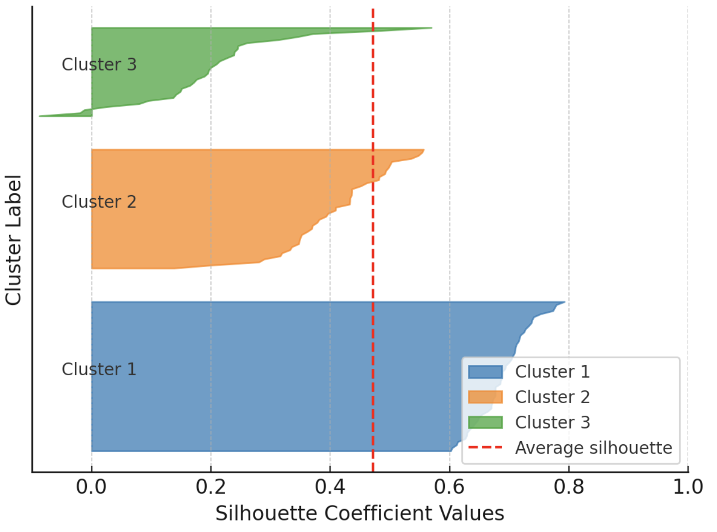
Instance visualization of silhouette scores
Picture by Writer
On the draw back, silhouette evaluation could also be much less dependable for sure datasets and cluster shapes (e.g., non-convex or intricately formed clusters) and may be difficult in very high-dimensional areas.
Silhouette Evaluation in Motion: The Penguins Dataset
As an instance cluster analysis utilizing silhouette evaluation, we’ll use the well-known Palmer Archipelago penguins dataset, particularly the model freely out there right here.
We rapidly stroll via the preparatory steps (loading and preprocessing), that are defined intimately on this introductory cluster evaluation tutorial. We’ll use pandas, scikit-learn, Matplotlib, and NumPy.
import pandas as pd
from sklearn.preprocessing import StandardScaler
from sklearn.cluster import KMeans
from sklearn.metrics import silhouette_score, silhouette_samples
import matplotlib.pyplot as plt
import numpy as np
# Load dataset (substitute with precise path or URL)
penguins = pd.read_csv(‘https://uncooked.githubusercontent.com/gakudo-ai/open-datasets/refs/heads/principal/penguins.csv’)
penguins = penguins.dropna()
options = [‘bill_length_mm’, ‘bill_depth_mm’, ‘flipper_length_mm’, ‘body_mass_g’]
X = penguins[features]
# Scale numerical options for more practical clustering
scaler = StandardScaler()
X_scaled = scaler.fit_transform(X)
1
2
3
4
5
6
7
8
9
10
11
12
13
14
15
16
17
import pandas as pd
from sklearn.preprocessing import StandardScaler
from sklearn.cluster import KMeans
from sklearn.metrics import silhouette_score, silhouette_samples
import matplotlib.pyplot as plt
import numpy as np
# Load dataset (substitute with precise path or URL)
penguins = pd.read_csv(‘https://uncooked.githubusercontent.com/gakudo-ai/open-datasets/refs/heads/principal/penguins.csv’)
penguins = penguins.dropna()
options = [‘bill_length_mm’, ‘bill_depth_mm’, ‘flipper_length_mm’, ‘body_mass_g’]
X = penguins[features]
# Scale numerical options for more practical clustering
scaler = StandardScaler()
X_scaled = scaler.fit_transform(X)
Subsequent, we apply k-means to search out clusters within the dataset. We repeat this course of for a number of values of the variety of clusters okay (the n_clusters parameter), starting from 2 to six. For every setting, we calculate the silhouette rating.
range_n_clusters = listing(vary(2, 7))
silhouette_avgs = []
for n_clusters in range_n_clusters:
kmeans = KMeans(n_clusters=n_clusters, n_init=10, random_state=42)
cluster_labels = kmeans.fit_predict(X_scaled)
sil_avg = silhouette_score(X_scaled, cluster_labels)
silhouette_avgs.append(sil_avg)
print(f”For n_clusters = {n_clusters}, common silhouette_score = {sil_avg:.3f}”)
range_n_clusters = listing(vary(2, 7))
silhouette_avgs = []
for n_clusters in range_n_clusters:
kmeans = KMeans(n_clusters=n_clusters, n_init=10, random_state=42)
cluster_labels = kmeans.fit_predict(X_scaled)
sil_avg = silhouette_score(X_scaled, cluster_labels)
silhouette_avgs.append(sil_avg)
print(f“For n_clusters = {n_clusters}, common silhouette_score = {sil_avg:.3f}”)
The ensuing output is:
For n_clusters = 2, common silhouette_score = 0.531
For n_clusters = 3, common silhouette_score = 0.446
For n_clusters = 4, common silhouette_score = 0.419
For n_clusters = 5, common silhouette_score = 0.405
For n_clusters = 6, common silhouette_score = 0.392
For n_clusters = 2, common silhouette_score = 0.531
For n_clusters = 3, common silhouette_score = 0.446
For n_clusters = 4, common silhouette_score = 0.419
For n_clusters = 5, common silhouette_score = 0.405
For n_clusters = 6, common silhouette_score = 0.392
This means that the very best silhouette rating is obtained for okay = 2. This often signifies essentially the most coherent grouping of the information factors, though it doesn’t at all times match organic or area floor reality.
Within the penguins dataset, though there are three species with distinct traits, repeated k-means clustering and silhouette evaluation point out that partitioning the information into two teams may be extra constant within the chosen function area. This will occur as a result of silhouette evaluation displays geometric separability within the chosen options (right here, 4 numeric attributes) somewhat than categorical labels; overlapping traits amongst species might lead k-means to favor fewer clusters than the precise variety of species.
Let’s visualize the silhouette outcomes for all 5 configurations:
fig, axes = plt.subplots(1, len(range_n_clusters), figsize=(25, 5), sharey=False)
for i, n_clusters in enumerate(range_n_clusters):
ax = axes[i]
kmeans = KMeans(n_clusters=n_clusters, n_init=10, random_state=42)
labels = kmeans.fit_predict(X_scaled)
sil_vals = silhouette_samples(X_scaled, labels)
sil_avg = silhouette_score(X_scaled, labels)
y_lower = 10
for j in vary(n_clusters):
ith_sil_vals = sil_vals[labels == j]
ith_sil_vals.type()
size_j = ith_sil_vals.form[0]
y_upper = y_lower + size_j
colour = plt.cm.nipy_spectral(float(j) / n_clusters)
ax.fill_betweenx(np.arange(y_lower, y_upper),
0, ith_sil_vals,
facecolor=colour, edgecolor=colour, alpha=0.7)
ax.textual content(-0.05, y_lower + 0.5 * size_j, str(j))
y_lower = y_upper + 10 # separation between clusters
ax.set_title(f”Silhouette Plot for okay = {n_clusters}”)
ax.axvline(x=sil_avg, colour=”purple”, linestyle=”–“)
ax.set_xlabel(“Silhouette Coefficient”)
if i == 0:
ax.set_ylabel(“Cluster Label”)
ax.set_xlim([-0.1, 1])
ax.set_ylim([0, len(X_scaled) + (n_clusters + 1) * 10])
plt.tight_layout()
plt.present()
1
2
3
4
5
6
7
8
9
10
11
12
13
14
15
16
17
18
19
20
21
22
23
24
25
26
27
28
29
30
31
32
33
fig, axes = plt.subplots(1, len(range_n_clusters), figsize=(25, 5), sharey=False)
for i, n_clusters in enumerate(range_n_clusters):
ax = axes[i]
kmeans = KMeans(n_clusters=n_clusters, n_init=10, random_state=42)
labels = kmeans.fit_predict(X_scaled)
sil_vals = silhouette_samples(X_scaled, labels)
sil_avg = silhouette_score(X_scaled, labels)
y_lower = 10
for j in vary(n_clusters):
ith_sil_vals = sil_vals[labels == j]
ith_sil_vals.type()
size_j = ith_sil_vals.form[0]
y_upper = y_lower + size_j
colour = plt.cm.nipy_spectral(float(j) / n_clusters)
ax.fill_betweenx(np.arange(y_lower, y_upper),
0, ith_sil_vals,
facecolor=colour, edgecolor=colour, alpha=0.7)
ax.textual content(–0.05, y_lower + 0.5 * size_j, str(j))
y_lower = y_upper + 10 # separation between clusters
ax.set_title(f“Silhouette Plot for okay = {n_clusters}”)
ax.axvline(x=sil_avg, colour=“purple”, linestyle=“–“)
ax.set_xlabel(“Silhouette Coefficient”)
if i == 0:
ax.set_ylabel(“Cluster Label”)
ax.set_xlim([–0.1, 1])
ax.set_ylim([0, len(X_scaled) + (n_clusters + 1) * 10])
plt.tight_layout()
plt.present()
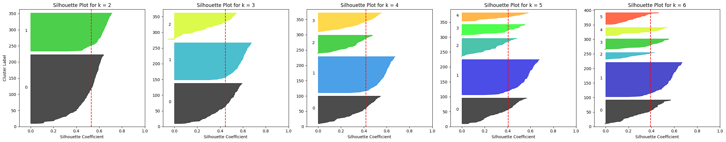
Silhouette plots for a number of k-means configurations on the Penguins dataset
Picture by Writer
One clear statement is that for okay ≥ 4 the typical silhouette rating drops to roughly 0.4, whereas it’s greater for okay = 2 or okay = 3.
What if we think about a special (narrower) subset of attributes for clustering? As an illustration, think about solely invoice size and flipper size. This is so simple as changing the function choice assertion close to the beginning of the code with:
options = [‘bill_length_mm’, ‘flipper_length_mm’]
options = [‘bill_length_mm’, ‘flipper_length_mm’]
Then rerun the remaining. Strive totally different function picks previous to clustering and test whether or not the silhouette evaluation outcomes stay comparable or differ for some decisions of the variety of clusters.
Wrapping Up
This text offered a concise, sensible understanding of a normal cluster-quality metric for clustering algorithms: the silhouette rating, and confirmed find out how to use it to research clustering outcomes critically.
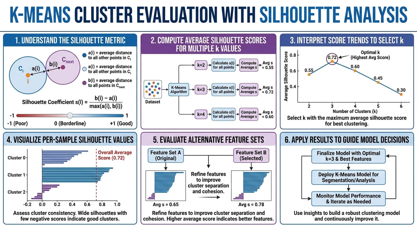
Okay-means cluster analysis with silhouette evaluation in six straightforward steps (click on to enlarge)