


On this tutorial, we’ll discover the scope of SHAP-IQ visualizations that present perception into how machine studying fashions attain their predictions. These visuals assist to interrupt down the habits of complicated fashions into interpretable parts. This reforms each particular person contributions of options and contributions to particular predictions. See the total code right here.
Dependencies Set up
Importing a dataset
This tutorial makes use of an MPG (mile per gallon) dataset. This hundreds straight from the Seaborn Library. This dataset accommodates details about numerous automotive fashions, together with options equivalent to horsepower, weight, and origin. See the total code right here.
Processing datasets
Utilizing label encoding, it converts categorical columns to numerical codecs, making them appropriate for mannequin coaching.
Break up the info into coaching and check subsets
feature_names = x.columns.tolist() x_data, y_data = x.values, y.values #traintest cut up x_train, x_test, y_train, y_test = train_test_split (x_data, y_data, test_size = 0.2, random_state=42)
Mannequin Coaching
Prepare random forest regression on resolution timber (N_ESTIMATORS = 10) with most depths of 10 and 10. A hard and fast RANDOM_STATE ensures repeatability.
Mannequin analysis
Native Occasion Description
Choose a selected check occasion (utilizing instance_id = 7) to research how the mannequin reached the prediction. Prints the true, predicted, and have values for this occasion. See the total code right here.
y_true = y_test[instance_id]
y_pred = mannequin.predict(x_explain.reshape(1,-1))[0]
print(f “occasion {instance_id}, true worth: {y_true}, predicted worth: {y_pred}”) i, function in enumerate (feature_names): print(f “{function}: {x_explain[i]} “)
Generates descriptions of a number of interplay orders
Use the Shapiq package deal to generate Shapley-based descriptions of various interplay orders. Particularly, calculate the next:
Order 1 (commonplace Shapley worth): Particular person function contribution order 2 (pairwise interplay): Perform pair mixture impact order n (full interplay): All interactions as much as the full variety of options
1. Energy Chart
Forceplots are highly effective visualization instruments that enable you perceive how machine studying fashions have reached a specific prediction. It shows baseline predictions (i.e., the anticipated values of the earlier mannequin earlier than trying on the function) and exhibits how every function makes the prediction greater or decrease.
On this plot:
Pink bars symbolize options or interactions that enhance prediction. A blue bar represents one thing that reduces it. The size of every bar corresponds to the scale of its impact.
When utilizing Shapley’s interplay values, the pressure plot can visualize interactions between features in addition to particular person contributions. That is significantly insightful when decoding complicated fashions. It’s because it visually breaks down how the mixtures of options work collectively to have an effect on the result. See the total code right here.
From the primary plot, we will see that the bottom worth is 23.5. Options equivalent to weight, cylinder, horsepower, and displacement have a optimistic impact on prediction and push it above the baseline. In the meantime, mannequin 12 months and acceleration have a adverse influence, pulling forecasts down.
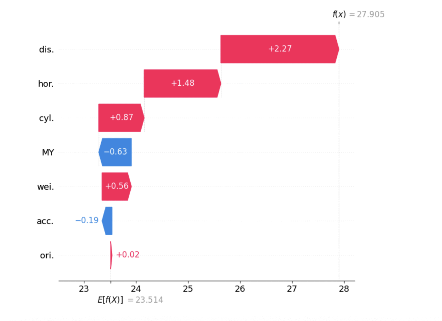
2. Waterfall Chart
Like pressure plots, waterfall plots are one other frequent option to visualize Shapley values initially launched within the Shap library. Varied options point out greater or decrease predictions in comparison with baseline. One of many key advantages of waterfall plots is that it mechanically group options which have very small influence on the “different” classes, making the chart cleaner and simpler to know. See the total code right here.


3. Community Plot
The community plot exhibits how options work together utilizing one Shapley interplay. The node measurement displays the influence of particular person options, whereas the sting width and shade point out the energy and orientation of the interplay. It’s particularly helpful when coping with many options, revealing complicated interactions that less complicated plots could miss. See the total code right here.

4. Si graph plot
SI graph plots prolong the community plot by visualizing all greater order interactions as hyperedges connecting a number of features. Node measurement signifies the affect of particular person options, whereas edge width, shade, and transparency mirror the depth and orientation of the interplay. This supplies a complete view of how options collaboratively have an effect on mannequin predictions. See the total code right here.


5. Barplot
The bar plot is tailor-made to the worldwide description. Different plots can be utilized regionally and globally, however bar plots summarise the general significance of options (or function interactions) by exhibiting imply absolute Shapley (or interactions) values for all cases. In Shapiq, we spotlight the traits that the interplay contributes most on common. See the total code right here.
explainer =shapiq.treeexplainer(mannequin = mannequin, max_order = 2, index = “k-sii”) for tqdm (vary (20)): x_explain = x_test[instance_id]
si = explader.clarify(x = x_explain)contrisations.append(si)shapiq.plot.bar_plot(contressations, feature_names = feature_names, present = true)

“Distance” and “Horsepower” are essentially the most influential options general. That’s, it has the strongest private affect on mannequin prediction. That is evident from the excessive imply absolute Shapley interplay values within the bar plot.
Moreover, trying on the secondary interplay (i.e. how the 2 features work together), the mix “horsepower x weight” and “distance x horsepower” point out necessary joint results. Their mixed attributions are roughly 1.4, indicating that these interactions play an necessary position in shaping mannequin predictions past people who contribute individually to mannequin predictions. This highlights the existence of nonlinear relations between features inside the mannequin.
See the total code right here. For tutorials, code and notebooks, please go to our GitHub web page. Additionally, be at liberty to observe us on Twitter. Do not forget to hitch 100K+ ML SubredDit and subscribe to our publication.

I’m a civil engineering graduate (2022) from Jamia Milia Islamia, New Delhi, and have a powerful curiosity in information science, significantly neural networks and purposes in quite a lot of fields.