


On this article, you’ll learn to full three beginner-friendly pc imaginative and prescient duties in Python — edge detection, easy object detection, and picture classification — utilizing extensively obtainable libraries.
Matters we are going to cowl embrace:
Putting in and organising the required Python libraries.
Detecting edges and faces with basic OpenCV instruments.
Coaching a compact convolutional neural community for picture classification.
Let’s discover these methods.
The Newbie’s Information to Laptop Imaginative and prescient with Python
Picture by Editor
Introduction
Laptop imaginative and prescient is an space of synthetic intelligence that provides pc programs the power to investigate, interpret, and perceive visible knowledge, specifically photos and movies. It encompasses every thing from classical duties like picture filtering, edge detection, and have extraction, to extra superior duties reminiscent of picture and video classification and sophisticated object detection, which require constructing machine studying and deep studying fashions.
Fortunately, Python libraries like OpenCV and TensorFlow make it doable — even for novices — to create and experiment with their very own pc imaginative and prescient options utilizing just some strains of code.
This text is designed to information novices fascinated by pc imaginative and prescient by means of the implementation of three basic pc imaginative and prescient duties:
Picture processing for edge detection
Easy object detection, like faces
Picture classification
For every process, we offer a minimal working instance in Python that makes use of freely obtainable or built-in knowledge, accompanied by the required explanations. You may reliably run this code in a notebook-friendly surroundings reminiscent of Google Colab, or regionally in your individual IDE.
Setup and Preparation
An vital prerequisite for utilizing the code supplied on this article is to put in a number of Python libraries. In the event you run the code in a pocket book, paste this command into an preliminary cell (use the prefix “!” in notebooks):
pip set up opencv-python tensorflow scikit-image matplotlib numpy
pip set up opencv–python tensorflow scikit–picture matplotlib numpy
Picture Processing With OpenCV
OpenCV is a Python library that gives a variety of instruments for effectively constructing pc imaginative and prescient functions—from fundamental picture transformations to easy object detection duties. It’s characterised by its pace and broad vary of functionalities.
One of many main process areas supported by OpenCV is picture processing, which focuses on making use of transformations to photographs, usually with two objectives: enhancing their high quality or extracting helpful data. Examples embrace changing shade photos to grayscale, detecting edges, smoothing to cut back noise, and thresholding to separate particular areas (e.g. foreground from background).
The primary instance on this information makes use of a built-in pattern picture supplied by the scikit-image library to detect edges within the grayscale model of an initially full-color picture.
from skimage import knowledge
import cv2
import matplotlib.pyplot as plt
# Load a pattern RGB picture (astronaut) from scikit-image
picture = knowledge.astronaut()
# Convert RGB (scikit-image) to BGR (OpenCV conference), then to grayscale
picture = cv2.cvtColor(picture, cv2.COLOR_RGB2BGR)
grey = cv2.cvtColor(picture, cv2.COLOR_BGR2GRAY)
# Canny edge detection
edges = cv2.Canny(grey, 100, 200)
# Show
plt.determine(figsize=(10, 4))
plt.subplot(1, 2, 1)
plt.imshow(grey, cmap=”grey”)
plt.title(“Grayscale Picture”)
plt.axis(“off”)
plt.subplot(1, 2, 2)
plt.imshow(edges, cmap=”grey”)
plt.title(“Edge Detection”)
plt.axis(“off”)
plt.present()
1
2
3
4
5
6
7
8
9
10
11
12
13
14
15
16
17
18
19
20
21
22
23
24
25
26
27
28
from skimage import knowledge
import cv2
import matplotlib.pyplot as plt
# Load a pattern RGB picture (astronaut) from scikit-image
picture = knowledge.astronaut()
# Convert RGB (scikit-image) to BGR (OpenCV conference), then to grayscale
picture = cv2.cvtColor(picture, cv2.COLOR_RGB2BGR)
grey = cv2.cvtColor(picture, cv2.COLOR_BGR2GRAY)
# Canny edge detection
edges = cv2.Canny(grey, 100, 200)
# Show
plt.determine(figsize=(10, 4))
plt.subplot(1, 2, 1)
plt.imshow(grey, cmap=“grey”)
plt.title(“Grayscale Picture”)
plt.axis(“off”)
plt.subplot(1, 2, 2)
plt.imshow(edges, cmap=“grey”)
plt.title(“Edge Detection”)
plt.axis(“off”)
plt.present()
The method utilized within the code above is straightforward, but it illustrates a quite common picture processing situation:
Load and preprocess a picture for evaluation: convert the RGB picture to OpenCV’s BGR conference after which to grayscale for additional processing. Capabilities like COLOR_RGB2BGR and COLOR_BGR2GRAY make this simple.
Use the built-in Canny edge detection algorithm to determine edges within the picture.
Plot the outcomes: the grayscale picture used for edge detection and the ensuing edge map.
The outcomes are proven under:
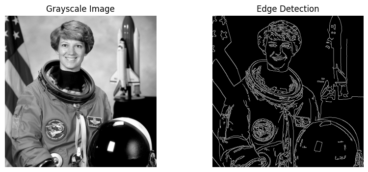
Edge detection with OpenCV
Object Detection With OpenCV
Time to transcend basic pixel-level processing and determine higher-level objects inside a picture. OpenCV makes this doable with pre-trained fashions like Haar cascades, which could be utilized to many real-world photos and work properly for easy detection use circumstances, e.g. detecting human faces.
The code under makes use of the identical astronaut picture as within the earlier part, converts it to grayscale, and applies a Haar cascade educated for figuring out frontal faces. The cascade’s metadata is contained in haarcascade_frontalface_default.xml.
from skimage import knowledge
import cv2
import matplotlib.pyplot as plt
# Load the pattern picture and convert to BGR (OpenCV conference)
picture = knowledge.astronaut()
picture = cv2.cvtColor(picture, cv2.COLOR_RGB2BGR)
# Haar cascade is an OpenCV classifier educated for detecting faces
face_cascade = cv2.CascadeClassifier(
cv2.knowledge.haarcascades + “haarcascade_frontalface_default.xml”
)
# The mannequin requires grayscale photos
grey = cv2.cvtColor(picture, cv2.COLOR_BGR2GRAY)
# Detect faces
faces = face_cascade.detectMultiScale(
grey, scaleFactor=1.1, minNeighbors=5
)
# Draw bounding containers
output = picture.copy()
for (x, y, w, h) in faces:
cv2.rectangle(output, (x, y), (x + w, y + h), (0, 255, 0), 2)
# Show
plt.imshow(cv2.cvtColor(output, cv2.COLOR_BGR2RGB))
plt.title(“Face Detection”)
plt.axis(“off”)
plt.present()
1
2
3
4
5
6
7
8
9
10
11
12
13
14
15
16
17
18
19
20
21
22
23
24
25
26
27
28
29
30
31
from skimage import knowledge
import cv2
import matplotlib.pyplot as plt
# Load the pattern picture and convert to BGR (OpenCV conference)
picture = knowledge.astronaut()
picture = cv2.cvtColor(picture, cv2.COLOR_RGB2BGR)
# Haar cascade is an OpenCV classifier educated for detecting faces
face_cascade = cv2.CascadeClassifier(
cv2.knowledge.haarcascades + “haarcascade_frontalface_default.xml”
)
# The mannequin requires grayscale photos
grey = cv2.cvtColor(picture, cv2.COLOR_BGR2GRAY)
# Detect faces
faces = face_cascade.detectMultiScale(
grey, scaleFactor=1.1, minNeighbors=5
)
# Draw bounding containers
output = picture.copy()
for (x, y, w, h) in faces:
cv2.rectangle(output, (x, y), (x + w, y + h), (0, 255, 0), 2)
# Show
plt.imshow(cv2.cvtColor(output, cv2.COLOR_BGR2RGB))
plt.title(“Face Detection”)
plt.axis(“off”)
plt.present()
Discover that the mannequin can return one or a number of detected objects (faces) in an inventory saved in faces. For each object detected, we extract the nook coordinates that outline the bounding containers enclosing the face.
End result:
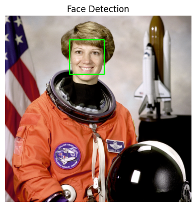
Face detection with OpenCV
Picture Classification With TensorFlow
Picture classification duties play in one other league. These issues are extremely depending on the precise dataset (or not less than on knowledge with related statistical properties). The primary sensible implication is that coaching a machine studying mannequin for classification is required. For easy, low-resolution photos, ensemble strategies like random forests or shallow neural networks might suffice, however for complicated, high-resolution photos, your finest wager is commonly deeper neural community architectures reminiscent of convolutional neural networks (CNNs) that study visible traits and patterns throughout courses.
This instance code makes use of the favored Vogue-MNIST dataset of low-resolution photos of garments, with examples distributed into 10 courses (shirt, trousers, sneakers, and so forth.). After some easy knowledge preparation, the dataset is partitioned into coaching and check units. In machine studying, the coaching set is handed along with labels (recognized courses for photos) so the mannequin can study the enter–output relationships. After coaching the mannequin — outlined right here as a easy CNN — the remaining examples within the check set could be handed to the mannequin to carry out class predictions, i.e. to deduce which kind of trend product is proven in a given picture.
import tensorflow as tf
from tensorflow.keras import layers, fashions
# Load Vogue-MNIST dataset (publicly obtainable)
(train_images, train_labels), (test_images, test_labels) =
tf.keras.datasets.fashion_mnist.load_data()
# Normalize pixel values for extra strong coaching
train_images = train_images.astype(“float32”) / 255.0
test_images = test_images.astype(“float32″) / 255.0
# Easy CNN structure with one convolution layer: sufficient for low-res photos
mannequin = fashions.Sequential([
layers.Reshape((28, 28, 1), input_shape=(28, 28)),
layers.Conv2D(32, 3, activation=”relu”),
layers.MaxPooling2D(),
layers.Flatten(),
layers.Dense(64, activation=”relu”),
layers.Dense(10, activation=”softmax”)
])
# Compile and practice the mannequin
mannequin.compile(
optimizer=”adam”,
loss=”sparse_categorical_crossentropy”,
metrics=[“accuracy”]
)
historical past = mannequin.match(
train_images,
train_labels,
epochs=5,
validation_split=0.1,
verbose=2
)
# (Optionally available) Consider on the check set
test_loss, test_acc = mannequin.consider(test_images, test_labels, verbose=0)
print(f”Check accuracy: {test_acc:.3f}”)
1
2
3
4
5
6
7
8
9
10
11
12
13
14
15
16
17
18
19
20
21
22
23
24
25
26
27
28
29
30
31
32
33
34
35
36
37
38
39
import tensorflow as tf
from tensorflow.keras import layers, fashions
# Load Vogue-MNIST dataset (publicly obtainable)
(train_images, train_labels), (test_images, test_labels) =
tf.keras.datasets.fashion_mnist.load_data()
# Normalize pixel values for extra strong coaching
train_images = train_images.astype(“float32”) / 255.0
test_images = test_images.astype(“float32”) / 255.0
# Easy CNN structure with one convolution layer: sufficient for low-res photos
mannequin = fashions.Sequential([
layers.Reshape((28, 28, 1), input_shape=(28, 28)),
layers.Conv2D(32, 3, activation=“relu”),
layers.MaxPooling2D(),
layers.Flatten(),
layers.Dense(64, activation=“relu”),
layers.Dense(10, activation=“softmax”)
])
# Compile and practice the mannequin
mannequin.compile(
optimizer=“adam”,
loss=“sparse_categorical_crossentropy”,
metrics=[“accuracy”]
)
historical past = mannequin.match(
train_images,
train_labels,
epochs=5,
validation_split=0.1,
verbose=2
)
# (Optionally available) Consider on the check set
test_loss, test_acc = mannequin.consider(test_images, test_labels, verbose=0)
print(f“Check accuracy: {test_acc:.3f}”)
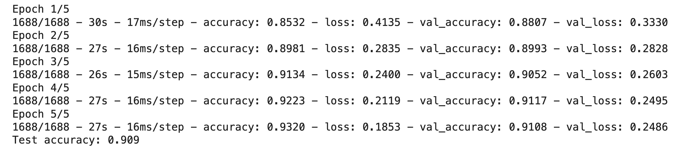
Coaching a picture classification with TensorFlow
And now you may have a educated mannequin.
Wrapping Up
This text guided novices by means of three widespread pc imaginative and prescient duties and confirmed easy methods to tackle them utilizing Python libraries like OpenCV and TensorFlow — from basic picture processing and pre-trained detectors to coaching a small predictive mannequin from scratch.