


On this article, you’ll learn the way MinMaxScaler, StandardScaler, and RobustScaler remodel skewed, outlier-heavy information, and find out how to decide the best one in your modeling pipeline.
Subjects we are going to cowl embrace:
How every scaler works and the place it breaks on skewed or outlier-rich information
A sensible artificial dataset to stress-test the scalers
A sensible, code-ready heuristic for selecting a scaler
Let’s not waste any extra time.
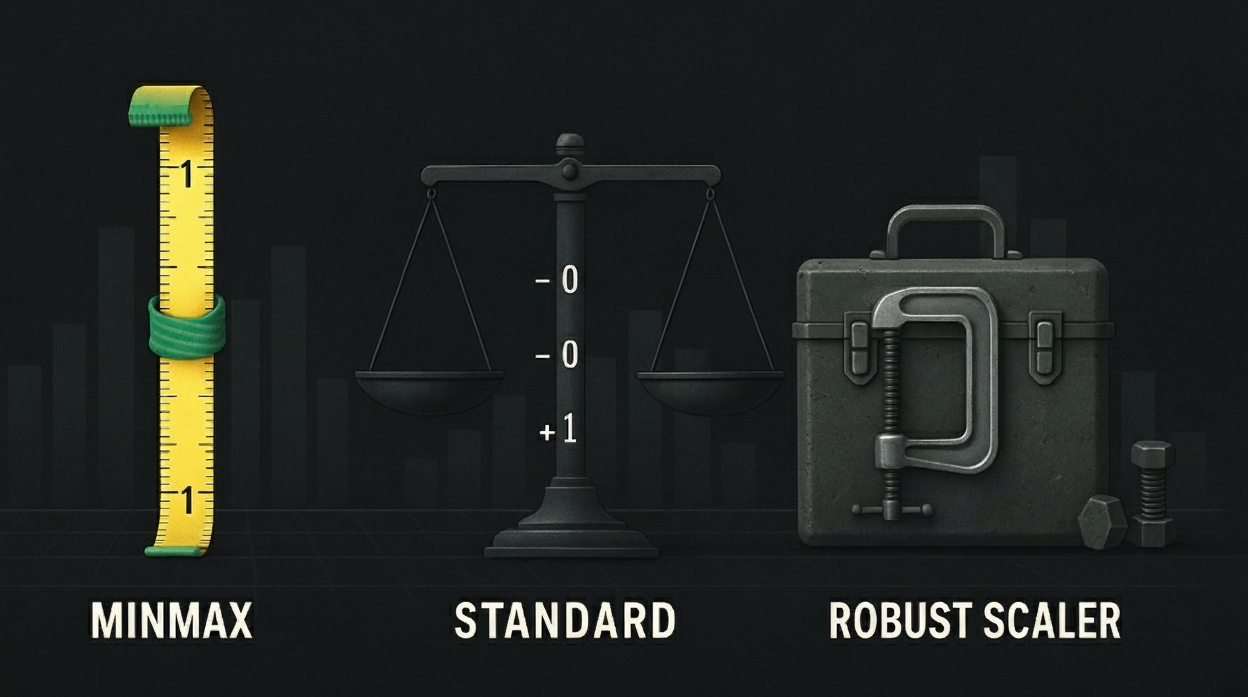
MinMax vs Commonplace vs Sturdy Scaler: Which One Wins for Skewed Knowledge?
Picture by Editor
Introduction
You’ve loaded your dataset and the distribution plots look tough. Heavy proper tail, some apparent outliers, and that acquainted sinking feeling that your mannequin efficiency is certain to be suboptimal. Been there?
Choosing the proper scaler for skewed information isn’t nearly following greatest practices. It’s about understanding what every methodology really does to your information and when these transformations assist versus damage your mannequin’s means to study significant patterns.
On this article, we’ll take a look at MinMaxScaler, StandardScaler, and RobustScaler on reasonable information, see precisely what occurs beneath the hood, and offer you a sensible choice framework in your subsequent mission. Let’s start!
🔗 Hyperlink to the code on GitHub
Understanding How Widespread Knowledge Scalers Work
Let’s begin by understanding how the completely different scalers work, their benefits and downsides.
MinMax Scaler
MinMax Scaler squashes every part into a set vary, often [0,1], utilizing your information’s minimal and most values.
scaled_value = (worth – min) / (max – min)
MinMaxScaler has the next benefits:
Bounded output vary [0,1]
Preserves authentic information relationships
Quick and easy to grasp
The issue: Excessive outliers make the denominator huge, compressing most of your precise information right into a tiny fraction of the accessible vary.
Commonplace Scaler
Commonplace Scaler facilities information round zero with unit variance by subtracting the imply and dividing by customary deviation.
scaled_value = (worth – imply) / standard_deviation
StandardScaler has the next benefits:
Works nice with usually distributed information
Facilities information round zero
Nicely-understood by most groups
The issue: Each imply and customary deviation are closely influenced by outliers, skewing the scaling for regular information factors.
Sturdy Scaler
Sturdy Scaler makes use of the median and interquartile vary (IQR) as a substitute of the imply and customary deviation, that are vulnerable to outliers.
scaled_value = (worth – median) / IQR
IQR = Q3 – Q1
the place:
Q1 = First quartile (twenty fifth percentile) – the worth under which 25% of information falls
Q3 = Third quartile (seventy fifth percentile) – the worth under which 75% of information falls
RobustScaler has the next benefits:
Immune to outliers
Makes use of percentiles (twenty fifth and seventy fifth) that ignore excessive values
Preserves information distribution form
The issue: It has an unbounded output vary, which might be much less intuitive to interpret.
Creating Pattern Knowledge
Let’s create a dataset that truly displays what you’ll encounter in manufacturing. We’ll mix three frequent information patterns: regular consumer habits, naturally skewed distributions (like income or web page views), and people excessive outliers that all the time appear to sneak into actual datasets. We’ll use NumPy, Pandas, Matplotlib, and SciPy.
import numpy as np
import pandas as pd
import matplotlib.pyplot as plt
from sklearn.preprocessing import MinMaxScaler, StandardScaler, RobustScaler
from scipy import stats
np.random.seed(42)
# Simulate typical consumer habits patterns
normal_data = np.random.regular(50, 15, 800)
# Add pure skew (frequent in income, pageviews, and so forth.)
skewed_data = np.random.exponential(2, 800) * 10 + 20
# Embody inevitable excessive outliers
outliers = [200, 180, 190, 210, 195]
# Mix into one messy dataset
information = np.concatenate([normal_data, skewed_data, outliers])
df = pd.DataFrame({‘authentic’: information})
# Apply all three scalers
scalers = {
‘MinMax’: MinMaxScaler(),
‘Commonplace’: StandardScaler(),
‘Sturdy’: RobustScaler()
}
for identify, scaler in scalers.gadgets():
df[name] = scaler.fit_transform(df[[‘original’]]).flatten()
# Examine what we’re working with
print(“Authentic Knowledge Stats:”)
print(f”Imply: {df[‘original’].imply():.2f}”)
print(f”Median: {df[‘original’].median():.2f}”)
print(f”Std Dev: {df[‘original’].std():.2f}”)
print(f”Skewness: {stats.skew(df[‘original’]):.2f}”)
print(f”Vary: {df[‘original’].min():.1f} to {df[‘original’].max():.1f}”)
1
2
3
4
5
6
7
8
9
10
11
12
13
14
15
16
17
18
19
20
21
22
23
24
25
26
27
28
29
30
31
32
33
34
35
36
37
38
import numpy as np
import pandas as pd
import matplotlib.pyplot as plt
from sklearn.preprocessing import MinMaxScaler, StandardScaler, RobustScaler
from scipy import stats
np.random.seed(42)
# Simulate typical consumer habits patterns
normal_data = np.random.regular(50, 15, 800)
# Add pure skew (frequent in income, pageviews, and so forth.)
skewed_data = np.random.exponential(2, 800) * 10 + 20
# Embody inevitable excessive outliers
outliers = [200, 180, 190, 210, 195]
# Mix into one messy dataset
information = np.concatenate([normal_data, skewed_data, outliers])
df = pd.DataFrame({‘authentic’: information})
# Apply all three scalers
scalers = {
‘MinMax’: MinMaxScaler(),
‘Commonplace’: StandardScaler(),
‘Sturdy’: RobustScaler()
}
for identify, scaler in scalers.gadgets():
df[name] = scaler.fit_transform(df[[‘original’]]).flatten()
# Examine what we’re working with
print(“Authentic Knowledge Stats:”)
print(f“Imply: {df[‘original’].imply():.2f}”)
print(f“Median: {df[‘original’].median():.2f}”)
print(f“Std Dev: {df[‘original’].std():.2f}”)
print(f“Skewness: {stats.skew(df[‘original’]):.2f}”)
print(f“Vary: {df[‘original’].min():.1f} to {df[‘original’].max():.1f}”)
Right here’s the information for the pattern dataset:
Authentic Knowledge Stats:
Imply: 45.65
Median: 42.81
Std Dev: 20.52
Skewness: 2.07
Vary: 1.4 to 210.0
Authentic Knowledge Stats:
Imply: 45.65
Median: 42.81
Std Dev: 20.52
Skewness: 2.07
Vary: 1.4 to 210.0
What Truly Occurs Throughout Knowledge Scaling
Let’s check out the numbers to grasp precisely what every scaler is doing to our information. The statistics will reveal why some scalers fail with skewed information whereas others deal with it fairly effectively.
Impact of MinMax Scaler on Pattern Knowledge
First, let’s study how MinMaxScaler’s reliance on min/max values creates issues when outliers are current.
print(“=== MinMaxScaler Evaluation ===”)
min_val = df[‘original’].min()
max_val = df[‘original’].max()
print(f”Scaling vary: {min_val:.1f} to {max_val:.1f}”)
# Present the compression impact
percentiles = [50, 75, 90, 95, 99]
for p in percentiles:
pct_val = df[‘MinMax’].quantile(p/100)
print(f”{p}% of information falls under: {pct_val:.3f}”)
data_below_half = (df[‘MinMax’] < 0.5).sum() / len(df) * 100
print(f”nResult: {data_below_half:.1f}% of information compressed under 0.5″)
print(“=== MinMaxScaler Evaluation ===”)
min_val = df[‘original’].min()
max_val = df[‘original’].max()
print(f“Scaling vary: {min_val:.1f} to {max_val:.1f}”)
# Present the compression impact
percentiles = [50, 75, 90, 95, 99]
for p in percentiles:
pct_val = df[‘MinMax’].quantile(p/100)
print(f“{p}% of information falls under: {pct_val:.3f}”)
data_below_half = (df[‘MinMax’] < 0.5).sum() / len(df) * 100
print(f“nResult: {data_below_half:.1f}% of information compressed under 0.5”)
Output:
=== MinMaxScaler Evaluation ===
Scaling vary: 1.4 to 210.0
50% of information falls under: 0.199
75% of information falls under: 0.262
90% of information falls under: 0.319
95% of information falls under: 0.368
99% of information falls under: 0.541
Outcome: 98.6% of information compressed under 0.5
=== MinMaxScaler Evaluation ===
Scaling vary: 1.4 to 210.0
50% of information falls under: 0.199
75% of information falls under: 0.262
90% of information falls under: 0.319
95% of information falls under: 0.368
99% of information falls under: 0.541
Outcome: 98.6% of information compressed under 0.5
What’s taking place: When outliers push the utmost to 210 whereas most information sits round 20-80, the denominator turns into large. The method (worth – min) / (max – min) compresses regular values right into a tiny fraction of the [0,1] vary.
Impact of Commonplace Scaler on Pattern Knowledge
Subsequent, let’s see how StandardScaler’s dependence on imply and customary deviation will get thrown off by outliers, affecting the scaling of completely regular information factors.
print(“n=== StandardScaler Evaluation ===”)
mean_orig = df[‘original’].imply()
std_orig = df[‘original’].std()
# Examine with/with out outliers
clean_data = df[‘original’][df[‘original’] < 150]
mean_clean = clean_data.imply()
std_clean = clean_data.std()
print(f”With outliers: imply={mean_orig:.2f}, std={std_orig:.2f}”)
print(f”With out outliers: imply={mean_clean:.2f}, std={std_clean:.2f}”)
print(f”Outlier influence: imply +{mean_orig – mean_clean:.2f}, std +{std_orig – std_clean:.2f}”)
# Present influence on typical information factors
typical_value = 50
z_with_outliers = (typical_value – mean_orig) / std_orig
z_without_outliers = (typical_value – mean_clean) / std_clean
print(f”nZ-score for worth 50:”)
print(f”With outliers: {z_with_outliers:.2f}”)
print(f”With out outliers: {z_without_outliers:.2f}”)
1
2
3
4
5
6
7
8
9
10
11
12
13
14
15
16
17
18
19
20
print(“n=== StandardScaler Evaluation ===”)
mean_orig = df[‘original’].imply()
std_orig = df[‘original’].std()
# Examine with/with out outliers
clean_data = df[‘original’][df[‘original’] < 150]
mean_clean = clean_data.imply()
std_clean = clean_data.std()
print(f“With outliers: imply={mean_orig:.2f}, std={std_orig:.2f}”)
print(f“With out outliers: imply={mean_clean:.2f}, std={std_clean:.2f}”)
print(f“Outlier influence: imply +{mean_orig – mean_clean:.2f}, std +{std_orig – std_clean:.2f}”)
# Present influence on typical information factors
typical_value = 50
z_with_outliers = (typical_value – mean_orig) / std_orig
z_without_outliers = (typical_value – mean_clean) / std_clean
print(f“nZ-score for worth 50:”)
print(f“With outliers: {z_with_outliers:.2f}”)
print(f“With out outliers: {z_without_outliers:.2f}”)
Output:
=== StandardScaler Evaluation ===
With outliers: imply=45.65, std=20.52
With out outliers: imply=45.11, std=18.51
Outlier influence: imply +0.54, std +2.01
Z-score for worth 50:
With outliers: 0.21
With out outliers: 0.26
=== StandardScaler Evaluation ===
With outliers: imply=45.65, std=20.52
With out outliers: imply=45.11, std=18.51
Outlier influence: imply +0.54, std +2.01
Z–rating for worth 50:
With outliers: 0.21
With out outliers: 0.26
What’s taking place: Outliers inflate each the imply and customary deviation. Regular information factors get distorted z-scores that misrepresent their precise place within the distribution.
Impact of Sturdy Scaler on Pattern Knowledge
Lastly, let’s display why RobustScaler’s use of the median and IQR makes it proof against outliers. This supplies constant scaling no matter excessive values.
print(“n=== RobustScaler Evaluation ===”)
median_orig = df[‘original’].median()
q25, q75 = df[‘original’].quantile([0.25, 0.75])
iqr = q75 – q25
# Examine with/with out outliers
clean_data = df[‘original’][df[‘original’] < 150]
median_clean = clean_data.median()
q25_clean, q75_clean = clean_data.quantile([0.25, 0.75])
iqr_clean = q75_clean – q25_clean
print(f”With outliers: median={median_orig:.2f}, IQR={iqr:.2f}”)
print(f”With out outliers: median={median_clean:.2f}, IQR={iqr_clean:.2f}”)
print(f”Outlier influence: median {abs(median_orig – median_clean):.2f}, IQR {abs(iqr – iqr_clean):.2f}”)
# Present consistency for typical information factors
typical_value = 50
robust_with_outliers = (typical_value – median_orig) / iqr
robust_without_outliers = (typical_value – median_clean) / iqr_clean
print(f”nRobust rating for worth 50:”)
print(f”With outliers: {robust_with_outliers:.2f}”)
print(f”With out outliers: {robust_without_outliers:.2f}”)
1
2
3
4
5
6
7
8
9
10
11
12
13
14
15
16
17
18
19
20
21
22
print(“n=== RobustScaler Evaluation ===”)
median_orig = df[‘original’].median()
q25, q75 = df[‘original’].quantile([0.25, 0.75])
iqr = q75 – q25
# Examine with/with out outliers
clean_data = df[‘original’][df[‘original’] < 150]
median_clean = clean_data.median()
q25_clean, q75_clean = clean_data.quantile([0.25, 0.75])
iqr_clean = q75_clean – q25_clean
print(f“With outliers: median={median_orig:.2f}, IQR={iqr:.2f}”)
print(f“With out outliers: median={median_clean:.2f}, IQR={iqr_clean:.2f}”)
print(f“Outlier influence: median {abs(median_orig – median_clean):.2f}, IQR {abs(iqr – iqr_clean):.2f}”)
# Present consistency for typical information factors
typical_value = 50
robust_with_outliers = (typical_value – median_orig) / iqr
robust_without_outliers = (typical_value – median_clean) / iqr_clean
print(f“nRobust rating for worth 50:”)
print(f“With outliers: {robust_with_outliers:.2f}”)
print(f“With out outliers: {robust_without_outliers:.2f}”)
Output:
=== RobustScaler Evaluation ===
With outliers: median=42.81, IQR=25.31
With out outliers: median=42.80, IQR=25.08
Outlier influence: median 0.01, IQR 0.24
Sturdy rating for worth 50:
With outliers: 0.28
With out outliers: 0.29
=== RobustScaler Evaluation ===
With outliers: median=42.81, IQR=25.31
With out outliers: median=42.80, IQR=25.08
Outlier influence: median 0.01, IQR 0.24
Sturdy rating for worth 50:
With outliers: 0.28
With out outliers: 0.29
What’s taking place: The median and IQR are calculated from the center 50% of information, so they continue to be secure even with excessive outliers. Regular information factors get constant scaled values.
When to Use Which Scaler
Based mostly on the understanding of how the completely different scalers work and their impact on a skewed dataset, right here’s a sensible choice framework I recommend:
Use MinMaxScaler when:
Your information has a recognized, significant vary (e.g., percentages, rankings)
You want bounded output for neural networks with particular activation features
No important outliers are current in your dataset
You’re doing picture processing the place pixel values have pure bounds
Use StandardScaler when:
Your information is roughly usually distributed
You’re utilizing algorithms that work effectively on information with zero imply and unit variance
No important outliers are corrupting imply/std deviation calculations
You need simple interpretation (values characterize customary deviations from the imply)
Use RobustScaler when:
Your information accommodates outliers that you may’t or shouldn’t take away
Your information is skewed however you need to protect the distribution form
You’re in exploratory phases and not sure about information high quality
You’re working with monetary, internet analytics, or different real-world messy information
Which Scaler to Select? Fast Choice Flowchart
Typically you want a fast programmatic method to decide on the best scaler. This operate analyzes your information’s traits and suggests probably the most applicable scaling methodology:
def recommend_scaler(information):
“””
Easy scaler suggestion primarily based on information traits
“””
# Calculate key statistics
skewness = abs(stats.skew(information))
q25, q75 = np.percentile(information, [25, 75])
iqr = q75 – q25
outlier_threshold = q75 + 1.5 * iqr
outlier_pct = (information > outlier_threshold).sum() / len(information) * 100
print(f”Knowledge evaluation:”)
print(f”Skewness: {skewness:.2f}”)
print(f”Outliers: {outlier_pct:.1f}% of information”)
if outlier_pct > 5:
return “RobustScaler – Excessive outlier proportion”
elif skewness > 1:
return “RobustScaler – Extremely skewed distribution”
elif skewness < 0.5 and outlier_pct < 1:
return “StandardScaler – Practically regular distribution”
else:
return “RobustScaler – Default secure alternative”
# Take a look at on our messy information
suggestion = recommend_scaler(df[‘original’])
print(f”nRecommendation: {suggestion}”)
1
2
3
4
5
6
7
8
9
10
11
12
13
14
15
16
17
18
19
20
21
22
23
24
25
26
27
def recommend_scaler(information):
“”“
Easy scaler suggestion primarily based on information traits
““”
# Calculate key statistics
skewness = abs(stats.skew(information))
q25, q75 = np.percentile(information, [25, 75])
iqr = q75 – q25
outlier_threshold = q75 + 1.5 * iqr
outlier_pct = (information > outlier_threshold).sum() / len(information) * 100
print(f“Knowledge evaluation:”)
print(f“Skewness: {skewness:.2f}”)
print(f“Outliers: {outlier_pct:.1f}% of information”)
if outlier_pct > 5:
return “RobustScaler – Excessive outlier proportion”
elif skewness > 1:
return “RobustScaler – Extremely skewed distribution”
elif skewness < 0.5 and outlier_pct < 1:
return “StandardScaler – Practically regular distribution”
else:
return “RobustScaler – Default secure alternative”
# Take a look at on our messy information
suggestion = recommend_scaler(df[‘original’])
print(f“nRecommendation: {suggestion}”)
As anticipated, RobustScaler works effectively on our pattern dataset.
Knowledge evaluation:
Skewness: 2.07
Outliers: 2.0% of information
Suggestion: RobustScaler – Extremely skewed distribution
Knowledge evaluation:
Skewness: 2.07
Outliers: 2.0% of information
Suggestion: RobustScaler – Extremely skewed distribution
Right here’s a easy flowchart that can assist you determine:

Picture by Writer | diagrams.internet (draw.io)
Conclusion
MinMaxScaler works nice when you will have clear information with pure boundaries. StandardScaler works effectively with usually distributed options however isn’t as efficient when outliers are current.
For many real-world datasets with skew and outliers, RobustScaler is your most secure guess when working with messy and skewed real-world information.
The perfect scaler is the one which preserves the significant patterns in your information whereas making them accessible to your chosen algorithm. There are lots of extra scalers whose implementations you will discover in scikit-learn for preprocessing skewed datasets.