


Language mannequin coaching is sluggish, even when your mannequin isn’t very massive. It’s because you have to practice the mannequin with a big dataset and there’s a massive vocabulary. Due to this fact, it wants many coaching steps for the mannequin to converge. Nonetheless, there are some strategies recognized to hurry up the coaching course of. On this article, you’ll study them. Specifically, you’ll study:
Utilizing optimizers
Utilizing studying fee schedulers
Different strategies for higher convergence or decreased reminiscence consumption
Let’s get began.
The way to Velocity-Up Coaching of Language Fashions
Photograph by Emma Fabbri. Some rights reserved.
Overview
This text is split into 4 elements; they’re:
Optimizers for Coaching Language Fashions
Studying Charge Schedulers
Sequence Size Scheduling
Different Strategies to Assist Coaching Deep Studying Fashions
Optimizers for Coaching Language Fashions
Adam has been the preferred optimizer for coaching deep studying fashions. In contrast to SGD and RMSProp, Adam makes use of each the primary and second second of the gradient to replace the parameters. Utilizing the second second can assist the mannequin converge quicker and extra stably, on the expense of utilizing extra reminiscence.
Nonetheless, when coaching language fashions these days, you’ll normally use AdamW, the Adam optimizer with weight decay. Weight decay is a regularization method to stop overfitting. It normally includes including a small penalty to the loss perform. However in AdamW, the burden decay is utilized on to the weights as an alternative. That is believed to be extra secure as a result of the regularization time period is decoupled from the calculated gradient. It’s also extra sturdy to hyperparameter tuning, because the impact of the regularization time period is utilized explicitly to the burden replace.
In formulation, AdamW weight replace algorithm is as follows:
$$
start{aligned}
g_t &= nabla_theta L(theta_{t-1})
m_t &= beta_1 m_{t-1} + (1 – beta_1) g_t
v_t &= beta_2 v_{t-1} + (1 – beta_2) g_t^2
hat{m_t} &= m_t / (1 – beta_1^t)
hat{v_t} &= v_t / (1 – beta_2^t)
theta_t &= theta_{t-1} – alpha Huge( frac{hat{m_t}}{sqrt{hat{v_t}} + epsilon} + lambda theta_{t-1} Huge)
finish{aligned}
$$
The mannequin weight at step $t$ is denoted by $theta_t$. The $g_t$ is the computed gradient from the loss perform $L$, and $g_t^2$ is the elementwise sq. of the gradient. The $m_t$ and $v_t$ are the transferring common of the primary and second second of the gradient, respectively. Studying fee $alpha$, weight decay $lambda$, and transferring common decay charges $beta_1$ and $beta_2$ are hyperparameters. A small worth $epsilon$ is used to keep away from division by zero. A standard alternative could be $beta_1 = 0.9$, $beta_2 = 0.999$, $epsilon = 10^{-8}$, and $lambda = 0.1$.
The important thing of AdamW is the $lambda theta_{t-1}$ time period within the gradient replace, as an alternative of within the loss perform.
AdamW isn’t the one alternative of optimizer. Some newer optimizers have been proposed not too long ago, corresponding to Lion, SOAP, and AdEMAMix. You’ll be able to see the paper Benchmarking Optimizers for Giant Language Mannequin Pretraining for a abstract.
Studying Charge Schedulers
A studying fee scheduler is used to regulate the educational fee throughout coaching. Normally, you would like a bigger studying fee for the early coaching steps and scale back the educational fee as coaching progresses to assist the mannequin converge. You’ll be able to add a warm-up interval to extend the educational fee from a small worth to the height over a brief interval (normally 0.1% to 2% of whole steps), then the educational fee is decreased over the remaining coaching steps.
A warm-up interval normally begins with a near-zero studying fee and will increase linearly to the height studying fee. A mannequin begins with randomized preliminary weights. Beginning with a big studying fee may cause poor convergence, particularly for giant fashions, massive batches, and adaptive optimizers.
You’ll be able to see the necessity for warm-up from the equations above. Assume the mannequin is uncalibrated; the loss might fluctuate significantly between subsequent steps. Then the primary and second moments $m_t$ and $v_t$ shall be fluctuating significantly, and the gradient replace $theta_t – theta_{t-1}$ can even be fluctuating significantly. Therefore, you would like the loss to be secure and transfer slowly in order that AdamW can construct a dependable operating common. This may be simply achieved if $alpha$ is small.
On the studying fee discount section, there are just a few selections:
cosine decay: $LR = LR_{max} cdot frac12 Huge(1 + cos frac{pi t}{T}Huge)$
square-root decay: $LR = LR_{max} cdot sqrt{frac{T – t}{T}}$
linear decay: $LR = LR_{max} cdot frac{T – t}{T}$
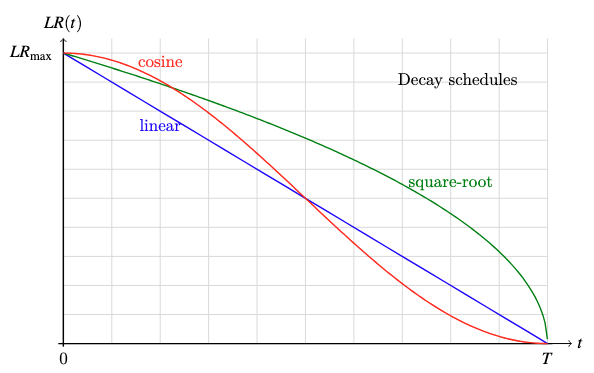
Plot of the three decay features
A big studying fee can assist the mannequin converge quicker whereas a small studying fee can assist the mannequin stabilize. Due to this fact, you need the educational fee to be massive at first when the mannequin remains to be uncalibrated, however small on the finish when the mannequin is near its optimum state. All decay schemes above can obtain this, however you wouldn’t need the educational fee to develop into “too small too quickly” or “too massive too late”. Cosine decay is the preferred alternative as a result of it drops the educational fee extra slowly at first and stays longer at a low studying fee close to the top, that are fascinating properties to assist the mannequin converge quicker and stabilize respectively.
n PyTorch, you’ve the CosineAnnealingLR scheduler to implement cosine decay. For the warm-up interval, you have to mix with the LinearLR scheduler. Beneath is an instance of the coaching loop utilizing AdamW, CosineAnnealingLR, and LinearLR:
import torch
import torch.nn as nn
import torch.optim as optim
from torch.optim.lr_scheduler import LinearLR, CosineAnnealingLR, SequentialLR
# Instance setup
mannequin = torch.nn.Linear(10, 1)
X, y = torch.randn(5, 10), torch.randn(5)
loss_fn = nn.MSELoss()
optimizer = optim.AdamW(mannequin.parameters(), lr=1e-2, betas=(0.9, 0.999), eps=1e-8, weight_decay=0.1)
# Outline studying fee schedulers
warmup_steps = 10
total_steps = 100
min_lr = 1e-4
warmup_lr = LinearLR(optimizer, start_factor=0.1, end_factor=1.0, total_iters=warmup_steps)
cosine_lr = CosineAnnealingLR(optimizer, T_max=total_steps – warmup_steps, eta_min=min_lr)
combined_lr = SequentialLR(optimizer, schedulers=[warmup_lr, cosine_lr], milestones=[warmup_steps])
# Coaching loop
for step in vary(total_steps):
# practice one epoch
y_pred = mannequin(X)
loss = loss_fn(y_pred, y)
# print loss and studying fee
print(f”Step {step+1}/{total_steps}: loss {loss.merchandise():.4f}, lr {combined_lr.get_last_lr()[0]:.4f}”)
# backpropagate and replace weights
optimizer.zero_grad()
loss.backward()
optimizer.step()
combined_lr.step()
1
2
3
4
5
6
7
8
9
10
11
12
13
14
15
16
17
18
19
20
21
22
23
24
25
26
27
28
29
30
31
import torch
import torch.nn as nn
import torch.optim as optim
from torch.optim.lr_scheduler import LinearLR, CosineAnnealingLR, SequentialLR
# Instance setup
mannequin = torch.nn.Linear(10, 1)
X, y = torch.randn(5, 10), torch.randn(5)
loss_fn = nn.MSELoss()
optimizer = optim.AdamW(mannequin.parameters(), lr=1e–2, betas=(0.9, 0.999), eps=1e–8, weight_decay=0.1)
# Outline studying fee schedulers
warmup_steps = 10
total_steps = 100
min_lr = 1e–4
warmup_lr = LinearLR(optimizer, start_factor=0.1, end_factor=1.0, total_iters=warmup_steps)
cosine_lr = CosineAnnealingLR(optimizer, T_max=total_steps – warmup_steps, eta_min=min_lr)
combined_lr = SequentialLR(optimizer, schedulers=[warmup_lr, cosine_lr], milestones=[warmup_steps])
# Coaching loop
for step in vary(total_steps):
# practice one epoch
y_pred = mannequin(X)
loss = loss_fn(y_pred, y)
# print loss and studying fee
print(f“Step {step+1}/{total_steps}: loss {loss.merchandise():.4f}, lr {combined_lr.get_last_lr()[0]:.4f}”)
# backpropagate and replace weights
optimizer.zero_grad()
loss.backward()
optimizer.step()
combined_lr.step()
Operating this code, you might even see:
Step 1/100: loss 1.5982, lr 0.0010
Step 2/100: loss 1.5872, lr 0.0019
Step 3/100: loss 1.5665, lr 0.0028
…
Step 9/100: loss 1.2738, lr 0.0082
Step 10/100: loss 1.2069, lr 0.0091
Step 11/100: loss 1.1387, lr 0.0100
…
Step 98/100: loss 0.4845, lr 0.0001
Step 99/100: loss 0.4845, lr 0.0001
Step 100/100: loss 0.4845, lr 0.0001
Discover how the educational fee will increase after which decreases.
Sequence Size Scheduling
Language fashions are educated with sequence knowledge. Transformer fashions or recurrent neural networks are each architecturally agnostic to the sequence size. Nonetheless, it’s possible you’ll need to practice the mannequin with lengthy sequence to let the mannequin discover ways to deal with lengthy context.
In coaching, lengthy sequence lengths may be problematic. First, you practice with batches of sequences, and ragged lengths imply you have to pad the sequences to the utmost size within the batch. Whereas you’ll ignore the padded tokens, your mannequin nonetheless must course of them, therefore assets are wasted. Second, within the consideration mechanism, the complexity is quadratic to the sequence size. The longer the sequence, the extra pricey it’s to course of.
Due to this fact, it’s possible you’ll need to create batches with sequences of comparable size to keep away from extreme padding.
You might also need to practice the mannequin with shorter sequences first. You’ll be able to velocity up the coaching course of by rapidly forcing the mannequin to study the patterns of the language utilizing shorter sequences. As soon as the mannequin has pretty converged, you possibly can steadily enhance the sequence size to assist the mannequin discover ways to deal with lengthy contexts.
These are widespread strategies in coaching massive language fashions to avoid wasting computational assets. Word that you simply nonetheless arrange the mannequin with a set most sequence size, which impacts the way you configure the positional embeddings. Nonetheless, you don’t exhaust the utmost sequence size till the mannequin has pretty converged.
Implementing sequence size scheduling means you have to write a extra complicated knowledge loader to consider of the present epoch to return the suitable coaching knowledge.
Different Strategies to Assist Coaching Deep Studying Fashions
Random Restart
Coaching a deep studying mannequin is a fancy course of and never simple to get proper, particularly for big fashions. One widespread subject is the mannequin getting caught in an area minimal and being unable to converge. Utilizing momentum in gradient descent can assist the mannequin escape from native minima, however isn’t all the time efficient. One other strategy is to easily restart the coaching should you ever see the mannequin fail to converge.
Random restart is the technique of coaching the mannequin a number of instances from scratch. It makes use of completely different random seeds every time in order that the mannequin begins with completely different preliminary weights and completely different shuffling of the information. That is completed within the hope that you’ll not all the time get caught in the identical native minimal, so you possibly can decide the one with one of the best efficiency. That is splendid should you can practice a number of fashions for fewer epochs at first, then decide one of the best mannequin from the pool to complete coaching with extra epochs.
Gradient Clipping
One widespread subject in coaching deep studying fashions is gradient explosion. That is particularly widespread should you practice the mannequin utilizing lower-precision floating-point numbers, by which the vary of the gradient could possibly be too massive to be represented. Gradient clipping is the strategy of limiting the magnitude of the gradient to a secure worth. With out it, you might even see your coaching course of all of a sudden fail as a result of mannequin weights or loss perform changing into NaN or infinity.
There are a number of methods to clip gradients. The commonest one is to clip the gradient such that the L2 norm is lower than a secure worth, corresponding to 1.0 or 6.0. It’s also possible to clip the gradient to a price vary, corresponding to -5.0 to five.0.
Gradient clipping by L2 norm means scaling the whole gradient vector if the L2 norm $Vert g_t Vert_2$ is larger than a secure worth $c$:
$$
hat{g_t} = minbig(1, frac{c}{Vert g_t Vert_2}massive) cdot g_t
$$
However, gradient clipping by worth means setting the gradient to a secure worth every time the gradient exceeds that worth:
$$
hat{g_t} = start{instances}
-c & textual content{if } g_t < -c
g_t & textual content{if } -c le g_t le c
c & textual content{if } g_t > c
finish{instances}
$$
Utilizing gradient clipping in PyTorch is simple. You need to use the torch.nn.utils.clip_grad_norm_ perform to clip the gradient by L2 norm, or the torch.nn.utils.clip_grad_value_ perform to clip the gradient by worth. Beneath is an instance:
import torch
import torch.nn as nn
import torch.optim as optim
from torch.nn.utils import clip_grad_norm_, clip_grad_value_
# Instance setup
mannequin = torch.nn.Linear(10, 1)
X, y = torch.randn(5, 10), torch.randn(5)
total_steps = 100
loss_fn = nn.MSELoss()
optimizer = optim.AdamW(mannequin.parameters(), lr=1e-2, betas=(0.9, 0.999), eps=1e-8, weight_decay=0.1)
# Coaching loop
for step in vary(total_steps):
# practice one epoch
y_pred = mannequin(X)
loss = loss_fn(y_pred, y)
optimizer.zero_grad()
loss.backward()
# clip by L2 norm
clip_grad_norm_(mannequin.parameters(), max_norm=1.0)
# or clip by worth
# clip_grad_value_(mannequin.parameters(), clip_value=1.0)
optimizer.step()
1
2
3
4
5
6
7
8
9
10
11
12
13
14
15
16
17
18
19
20
21
22
23
24
import torch
import torch.nn as nn
import torch.optim as optim
from torch.nn.utils import clip_grad_norm_, clip_grad_value_
# Instance setup
mannequin = torch.nn.Linear(10, 1)
X, y = torch.randn(5, 10), torch.randn(5)
total_steps = 100
loss_fn = nn.MSELoss()
optimizer = optim.AdamW(mannequin.parameters(), lr=1e–2, betas=(0.9, 0.999), eps=1e–8, weight_decay=0.1)
# Coaching loop
for step in vary(total_steps):
# practice one epoch
y_pred = mannequin(X)
loss = loss_fn(y_pred, y)
optimizer.zero_grad()
loss.backward()
# clip by L2 norm
clip_grad_norm_(mannequin.parameters(), max_norm=1.0)
# or clip by worth
# clip_grad_value_(mannequin.parameters(), clip_value=1.0)
optimizer.step()
Blended Precision Coaching
When a mannequin turns into too massive, reminiscence consumption turns into a bottleneck as nicely. Chances are you’ll need to save reminiscence through the use of lower-precision floating-point numbers in coaching, corresponding to half precision (float16) or bfloat16. In comparison with single precision (float32), float16 and bfloat16 can scale back reminiscence consumption by half, however the vary and precision are sacrificed.
Due to this fact, it’s possible you’ll need to use combined precision coaching, by which a part of the mannequin makes use of float32 whereas the opposite half makes use of float16. A standard alternative is to make use of float32 for biases however float16 for weights in linear layers.
Trendy GPUs can run float16 operations on the identical velocity as float32, however since you possibly can function on extra knowledge on the identical time, you possibly can successfully run the coaching course of at double velocity.
Additional Readings
Beneath are some assets that you could be discover helpful:
Abstract
On this article, you discovered about some strategies to hurry up the coaching technique of deep studying fashions, particularly for big language fashions. Particularly, you discovered that:
AdamW with cosine decay is the preferred optimizer and studying fee scheduler for coaching language fashions.
You need to use sequence size scheduling to avoid wasting computational assets when coaching language fashions.
Strategies like random restart and gradient clipping can assist you practice the mannequin extra stably.
Blended precision coaching can assist you scale back reminiscence consumption.