


On this article, learn to choose an applicable time collection forecasting mannequin utilizing a well-defined four-quadrant choice matrix based mostly on knowledge complexity and enter dimensionality.
Subjects lined embody:
The distinction between univariate and multivariate time collection and why it issues. Which classical and trendy fashions finest match low-complexity and high-complexity knowledge? Tradeoffs between interpretability, scalability, and accuracy throughout mannequin households.
Let’s not waste any extra time.
Determination matrix for time collection forecasting fashions
Picture by editor
introduction
Time collection knowledge provides complexity as a consequence of temporal dependencies, seasonality, and potential non-stationarity.
Maybe essentially the most frequent forecasting downside addressed with time collection knowledge is forecasting, or predicting the long run worth of variables reminiscent of temperature or inventory costs based mostly on historic observations so far. With so many alternative fashions for time collection forecasting, practitioners can typically discover it tough to decide on one of the best method.
This text is designed that can assist you by the usage of choice matrices with explanations of when and why to make use of completely different fashions relying on the traits of your knowledge and the kind of downside.
choice matrix
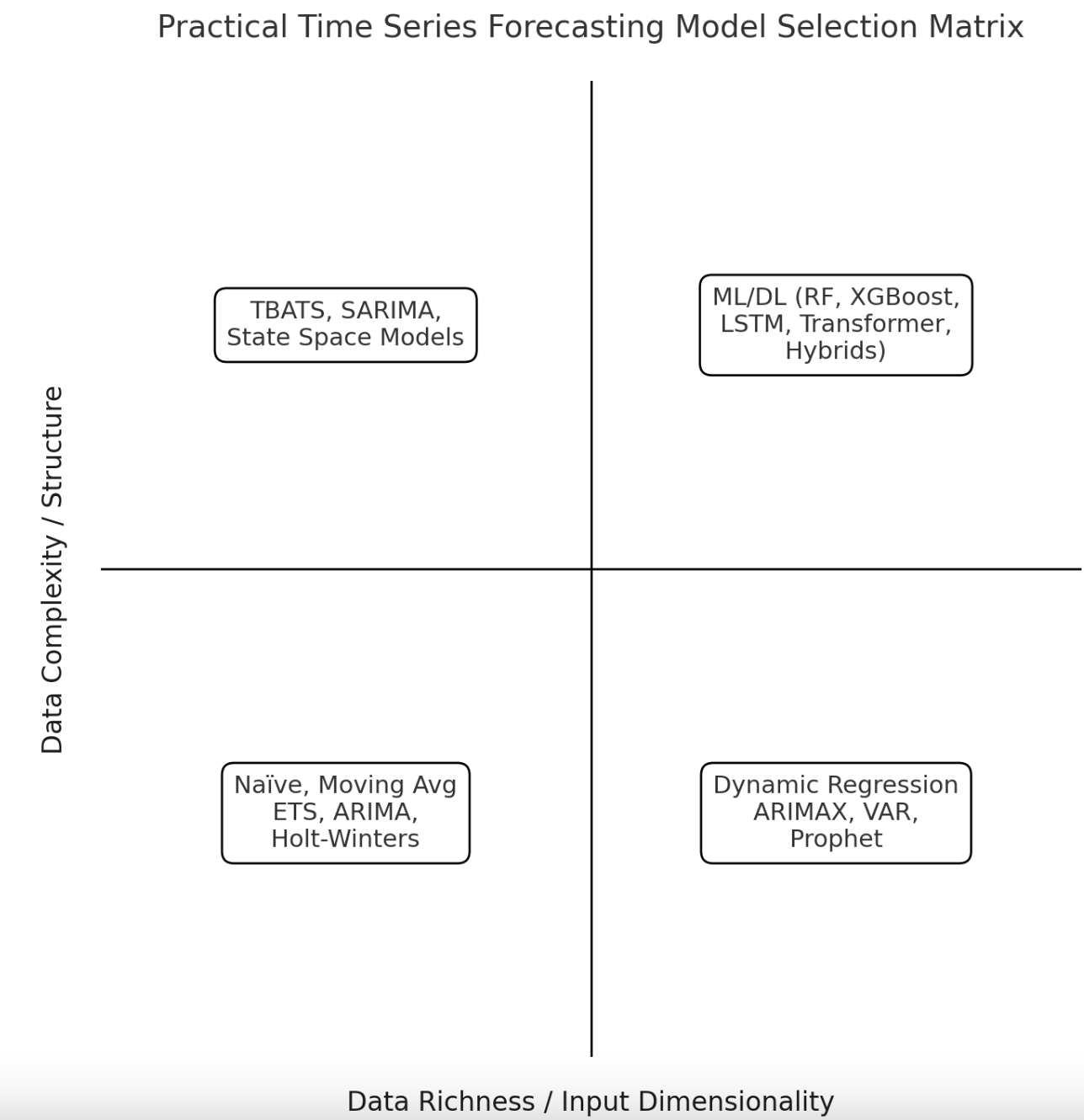
First, we introduce a visible matrix that classifies a set of generally used time collection forecasting fashions based mostly on two fundamental standards or dimensions.
Determination matrix for time collection forecasting fashions
Picture by creator
Knowledge complexity and construction refers back to the total complexity of the time collection dataset used by way of the presence or absence of stationary patterns, seasonality, restricted and important noise within the knowledge, nonlinearity, and many others.
Enter dimensionality refers to the truth that the time collection may be univariate or multivariate based mostly on the dimensionality of the enter knowledge. That’s, they might or might not have exogenous enter attributes, respectively. For instance, a dataset describing each day ridership on public transportation is an instance of a univariate time collection, whereas a each day or hourly climate file containing wind velocity, temperature, and humidity is an instance of a multivariate time collection.
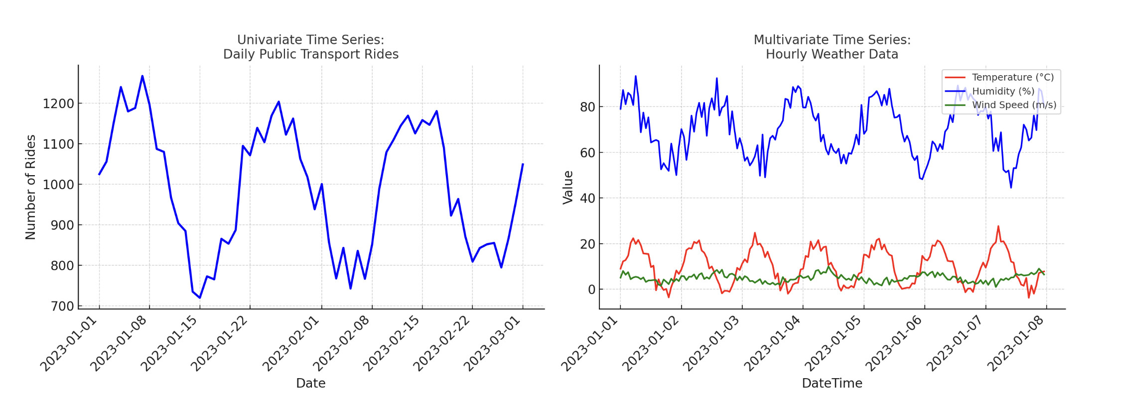
Univariate and multivariate time collection
Picture by creator
These two classification standards result in the classification of time collection forecasting fashions alongside the matrix proven above.
Let’s take a more in-depth take a look at every of the 4 quadrants.
1. Low-complexity univariate time collection (backside left)
This quadrant consists of forecasting issues when the complexity of the historic time collection is low. For instance, as a result of the time interval is pretty brief, the demand is steady (roughly fixed over time), or it reveals a easy pattern, sample, or seasonal construction. Sometimes, any such time collection additionally displays approximate stationarity.
Good easy fashions which might be normally adequate for these issues embody Naïve (for quite simple time collection knowledge), or barely extra complicated algorithms or methods reminiscent of transferring averages and their variants (easy transferring common, weighted transferring common), the traditional of classics, autoregressive built-in transferring common (ARIMA), and Holt-Winters. These are all sturdy fashions for easy time collection datasets whereas sustaining predictive interpretability and effectivity. Then again, as a consequence of its simplicity in comparison with different superior approaches, its adaptability to issues reminiscent of structural injury and exterior components could be very restricted.
2. Low-complexity multivariate time collection (backside proper)
In case your time collection nonetheless has a easy sample however is multivariate, or is influenced by a number of exterior components or regression predictors, chances are you’ll need to resort to fashions of average complexity reminiscent of dynamic regression, ARIMA with exogenous variables (ARIMAX), vector autoregression (VAR), or Prophet. These predictive fashions can incorporate recognized components reminiscent of promotions and pricing results in buyer previous behavioral knowledge immediately into their predictions, thereby appearing as a hybrid of purely time-based predictive and regression fashions.
These approaches are typically simple to interpret and implement, and produce dependable predictions if the underlying dynamics of the dataset stay comparatively easy. Then again, though they will incorporate exterior variables, they assume comparatively easy patterns and relationships and may battle with nonlinearities and difficult-to-understand interactions between variables.
3. Extremely complicated univariate time collection (high left)
Univariate time collection that exhibit complicated patterns reminiscent of irregular developments or a number of seasonal cycles require the usage of specialised fashions reminiscent of state-space methods reminiscent of TBATS (trigonometric features, Field-Cox transformation, ARMA error, pattern, and seasonal parts), seasonal ARIMA (SARIMA), or Kalman filter-based approaches. Elements reminiscent of non-stationarity, i.e. statistical properties of knowledge that change over time and complicated seasonal habits, may be captured by these fashions, making them appropriate for forecasting in long-term or irregular collection eventualities with considerably “unpredictable” dynamics.
Though these strategies are higher than different fashions in coping with inside complexity, they’re computationally intensive and in observe usually require cautious fine-tuning to be correct and generalizable.
4. Extremely complicated multivariate time collection (high proper)
The final of the 4 eventualities has a context with a big time collection that features a number of time and exterior variables and displays complicated or nonlinear dependencies. These tough eventualities require superior methods from the fields of machine studying and deep studying. Examples embody ensemble strategies reminiscent of random forests and XGBoost, recurrent neural networks reminiscent of lengthy short-term reminiscence (LSTM) networks, and even deep studying architectures reminiscent of transformers. However, in such conditions, utilizing a hybrid method is commonly a smart alternative.
These data-intensive fashions excel at capturing complicated interactions between variables and are scalable to very massive datasets. Nevertheless, the draw back is that it has extra stringent necessities, much less interpretability, and the chance of overfitting if adequate high-quality knowledge is just not offered for coaching.
abstract
This text mentioned time collection forecasting fashions and strategies from a sensible choice perspective. Based mostly on a four-quadrant choice matrix, we’ve got outlined the popular strategies to be used in 4 various kinds of forecasting eventualities, highlighted when to make use of every group of fashions, and outlined the strengths and weaknesses of every.